| |
Artículo original
Evaluation of richness in microbial communities
Evaluación de riqueza en comunidades microbianas
Cristóbal R. SANTA MARÍA 1 y Marcelo A. SORIA 2
1Departamento de Ingeniería e Investigaciones Tecnológicas. Universidad Nacional de La Matanza. 1754. San Justo. Argentina. csanta_maria@ing.unlam.edu.ar
2 Cátedra de Microbiología Agrícola. Facultad de Agronomía. Universidad de Buenos Aires. 1417. Buenos Aires. Argentina. soria@agro.uba.ar
Abstract:
Motivation: The richness of a microbial community is an important parameter to compare its structure with those of other communities across time and environments. The estimation of richness based on marker gene data obtained through Next Generation Sequencing faces several statistical problems. The current estimators, which are mostly derived for the analysis of macro-organisms, tend to grossly underestimate the richness of microbial communities. We developed a stochastic process to understand the effect of the structure of the population on the traditional richness estimators and introduce a new measure, the Algorithm for Quantifying Species (AQS)
Results: The AQS is a non-parametric estimator based on simulation that in our tests outperformed the traditional richness estimators, especially in the case of samples that are a very small fraction of the population and a large number of rare species, which is the frequent situation in metagenomics.
Resumen:
Motivación: La riqueza de una comunidad microbiana es un importante parámetro para comparar su estructura con otras comunidades a través del tiempo y el entorno. La estimación de la riqueza basada en datos de un gen marcador obtenidos por Secuenciación de Nueva Generación presenta diversos problemas estadísticos. Los estimadores habituales, derivados del análisis de macro-organismos, tienden a subestimar la riqueza de comunidades microbianas. Desarrollamos aquí un proceso estocástico para entender los efectos de la estructura de la población sobre las estimaciones tradicionales de riqueza e introducimos el Algoritmo de Recuento de Especies (AQS).
Resultados: AQS es un estimador no paramétrico basado en la simulación que en los test realizados mejora la estimación tradicional de la riqueza, especialmente en muestras que son muy pequeñas fracciones de la población y que contienen un gran número de especies raras, lo que es una situación frecuente en metagenómica.
Key Words: Estimation, Richness, DNA, Community .
Palabras Clave: Estimación, Riqueza, ADN, Comunidad.
I. INTRODUCTION
The quantification of the biodiversity in microbial communities is a complex task since, in addition to the statistical problems that arise similar to those found in the inference of richness or diversity in other kind of populations (Magurran, 2011), biases also emerge due to the process of metagenomic DNA, from which different individuals are identified, (Schloss, 2010; Youssef and Elshahed, 2008; Huse et al., 2010). This work is limited to explore an exper-imental methodology to treat the statistical inference of the popula-tion richness, and it supposes solved or at least mitigated by appro-priate precautions, the effects of the sequencing, alignment, filtering and any other process of DNA obtained from a community sample.
The technique used for microbial richness measurements requires a marker gene, highly conserved through evolution (Schloss-Handelsman 2006). Thus, when the sequences belonging to indi-viduals of the same sample reveal a certain percentage of variations between them, such variations can be attributed to the difference in species and, in general, in taxa, and not simply to random occurrences.
The sample once transformed into a set of marker gene sequences, it can be inferred through it, the richness of the community and perhaps also its distribution. This is where a significant statistical problem appears, since usually the sample size is insufficient for the task and, in the facts the richness is underestimated (Hughes et al., 2001). This is due to the presence of a significant proportion of rare species or taxa, in statistical terms, making it very unlikely to find in the sample individuals belonging to all or nearly all of them. Individuals of rare species are very few in relation to individuals of abundant species in the community and also rare species occur in greater numbers than the abundant species, so the sample size should be very large to infer a reasonably approximate value of the richness. In other words, the rarity and distribution of species seriously complicate the estimation of the population richness (Roesch, L. et al. 2007). This problem has been attempted to address by building parametric estimators as CHAO (Chao 1984) and ACE (Chao-Lee 1992) that even though they have improved the estimations they have not solved the inference, at least when it comes to microbial populations.
One line of current work (Haegeman et al., 2013) considers that the appropriate biodiversity assessment requires the analysis of a set of Hill indices that represent richness, entropy, etc. (Hill 1973) ( O´Hara, R. 2005). This perspective is expanded with the devel-opment of extrapolating rarefaction curves to assess the richness (Chao et al. 2014). The present work proposes an alternative pro-cedure to those mentioned by building a random process that is increasing the sample size in a simulated form, by using an estima-tion of the probability that, given a sample of size n, an upcoming individual who is added to the sample corresponds to a new species. This estimation was reported by Alan Turing in 1941 (Good 1953), (Nadas 1985).
Thus the Algorithm for Quantifying Species (AQS) designed updates the number of individuals and species in each iteration and grows the number of species simultaneously with the decrease to zero of the probability of finding a new species. Although the resulting distribution statistically may not correspond with the actual of the population, tests from samples of simulated and real populations allow seeing that, with a previous processing of the sequences to mitigate any bias, richness is better appreciated. This method of experimental modeling of the community can be com-putationally feasible and reasonable by optimizing execution times and with processing capabilities in parallel.
II. MATERIALS AND METHODS
1- In metagenomics, properties of a community are analyzed from the genomes of the individuals who composed it. In particular, given a microbial community, it is possible to sample and process the DNA to obtain sequences of the chosen marker gene that, in the present work, is the 16S rRNA (Armougom and Raoult 2009). Each sequence of this gene then corresponds to a distinct individual that integrates the sample and it is possible to gather sequences according to proximity criteria evaluated by the model of genetic distance of Jukes-Cantor or another similar (Hillis et al. 1996). Then, a threshold of dissimilarity between sequences can be taken, from which they will be considered as different species (or generally taxa). So different clusters are created that represent each one a species (or taxon) composed of individuals within the sample and are similar according to the threshold chosen (Schloss-Handelsman 2005). The n original sequences of the sample are distributed in clusters called Operational Taxonomic Units (OTU) and thus it can be built the distribution of sample abundance that indicates how many clusters contain r individuals, being  (Hill et al. 2003). (Hill et al. 2003).
To randomly select n individuals in a community that contains a finite and unknown number of species S, quantities  are, in each case, the number of species that records r individuals among the n selected. So are, in each case, the number of species that records r individuals among the n selected. So  . .
Clearly,  represents the number of species not represented by any of the n chosen individuals and the number of species in the community is represents the number of species not represented by any of the n chosen individuals and the number of species in the community is  .If the number of species recorded by taking n individuals is called .If the number of species recorded by taking n individuals is called  , then , then  (Chao and Shen. 2003). It is important to note that when adding a new individual to a sample, it may belong to an already present species or a new still unaccounted for. (Chao and Shen. 2003). It is important to note that when adding a new individual to a sample, it may belong to an already present species or a new still unaccounted for.
2- The method of rarefaction curves allows estimating the richness of a medium although it is generally applied to compare richness between two or more communities, because it relieves the problems arising from inadequate and usually unequal samples size (Hughes-Hellmann 2005) (Gotelli and Colwell. 2001). The basic idea of the rarefaction by individuals when trying to estimate the richness is that from taking larger samples is possible to capture an increasing number of different species. Given a community with an unknown number of individuals and a number S of different species also unknown, you can take samples of size n and determine  , which is the number of different species found in the sample. At each rearrangement that is carried out in the sample by examining each individual, the number of detected species will grow cumulatively according to the dotted curve in Figure 1. Once recorded i of the n individuals in each reordering, the expected theoretical value of , which is the number of different species found in the sample. At each rearrangement that is carried out in the sample by examining each individual, the number of detected species will grow cumulatively according to the dotted curve in Figure 1. Once recorded i of the n individuals in each reordering, the expected theoretical value of  is approximated by the average of the is approximated by the average of the  obtained for each of them. The curve formed by the points obtained for each of them. The curve formed by the points  , which is drawn in a continuous line in Figure 1, is called of rarefaction and can be used to estimate the S richness of the medium. , which is drawn in a continuous line in Figure 1, is called of rarefaction and can be used to estimate the S richness of the medium.
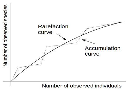 Fig. 1. The line of points is any Accumulation Curve. The complete line is a Rarefaction Curve.
The rarefaction curve represents the average of all accumulation curves built for different resamplings. When the number i=n of examined individuals is reached, any accumulation curve will have reached the number of species present in the sample size and therefore .
If n also results large enough, the rarefaction curve would tend asymptotically to the value of the richness population S. That is; to determine the horizontal asymptote of a rarefaction curve the sample size should be increased until  observes a steady behavior as n grows and in such circumstance the amount approximates the population richness S. observes a steady behavior as n grows and in such circumstance the amount approximates the population richness S.
3- An experimental model is built through a random process defined as follows:
Definition 1: Given a sample of size n, being, for each i with , the random variable that takes the values  and and 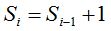 with the respective probabilities with the respective probabilities  and and  being also . The succession of random variables is hereinafter referred as Random Process of the Quantity of Species (Figure 2). being also . The succession of random variables is hereinafter referred as Random Process of the Quantity of Species (Figure 2).
The interpretation of the experimental model identifies  as the number of different species present in a sample of size n+i. In addition, is interpreted as the probability of that by incorporating a new individual to a sample of size , this one corresponds to a new species not present so far in the sample. It has been proved (Good 1953) that the probability that, once chosen n individuals, by selecting a new one it results to be from a species so far unaccounted for, this can be approximated by the quotient where as the number of different species present in a sample of size n+i. In addition, is interpreted as the probability of that by incorporating a new individual to a sample of size , this one corresponds to a new species not present so far in the sample. It has been proved (Good 1953) that the probability that, once chosen n individuals, by selecting a new one it results to be from a species so far unaccounted for, this can be approximated by the quotient where  is the number of species that appears once in the chosen sample and it must be assumed strictly greater than 0. is the number of species that appears once in the chosen sample and it must be assumed strictly greater than 0.
 Fig. 2. Random Process of the Quantity of Species.
This idea, provided by Turing, is used here to estimate  . Then, the proposed formula for calculating the probability of a new species associated with the random process of the quantity of species is . Then, the proposed formula for calculating the probability of a new species associated with the random process of the quantity of species is 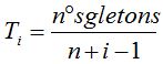 (Table 1). The number of singletons in each sample of size refers to the clusters formed by a single individual, when the sequences grouping process and the subsequent identification of each cluster with a different species are performed. (Table 1). The number of singletons in each sample of size refers to the clusters formed by a single individual, when the sequences grouping process and the subsequent identification of each cluster with a different species are performed.
Thus the expected value of Si that would correspond to the rarefaction curve when i simulated individuals have been added to the sample is: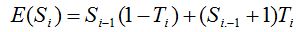 and operating is obtained. and operating is obtained.
Figure 3 shows how the probability of new species tends to zero, , as it grows the number of individuals incorporated to the sample by the simulation according to the experimental model. As the desired number of species S is finite (Good 1953), the rarefaction curve should be reaching an asymptote that estimates it.
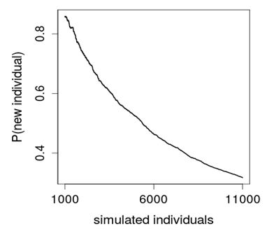 Fig. 3. Decreased Probability of New Species
The value of T in each iteration must be considered to be an estimation of the probability of a new species and not exactly this probability. Therefore, the expected value  will be only an approximate estimation of S. Thus the built model will be appropriate if the computational experience shows a good performance in the evaluation of S. In the practice, with the idea of reducing the variance, the same calculation from the same sample can be realized several times and it might average the quantities estimated. will be only an approximate estimation of S. Thus the built model will be appropriate if the computational experience shows a good performance in the evaluation of S. In the practice, with the idea of reducing the variance, the same calculation from the same sample can be realized several times and it might average the quantities estimated.
4- The Algorithm for Quantifying Species (AQS) is based on the Random Process of the Quantity of Species defined above. This algorithm performs the simulation by the Monte Carlo technique. Given the n size of the original sample, the value of the probability of new species estimator is determined. This value allows constituting the  and and  intervals so that when choosing a random number r such that , if it falls within the first interval the new simulated individual belongs to a new species, and if it falls within the second interval it is a specimen of a known species. If the former occurs, the number of species in the medium is increased in 1 and if not, the existing proportions of each species are used to assign, by a new random number, the already known species to which the new individual belongs. Thus individuals are added until the account of the new species reaches a stable value or until it meets another cutting criterion of the simulation. The procedural steps are synthesized in a sequenced form below. intervals so that when choosing a random number r such that , if it falls within the first interval the new simulated individual belongs to a new species, and if it falls within the second interval it is a specimen of a known species. If the former occurs, the number of species in the medium is increased in 1 and if not, the existing proportions of each species are used to assign, by a new random number, the already known species to which the new individual belongs. Thus individuals are added until the account of the new species reaches a stable value or until it meets another cutting criterion of the simulation. The procedural steps are synthesized in a sequenced form below.
i. Given the chosen sample of size n, and its grouping in OTUs, the initial value of the Turing estimator is determined, being  and the current number of singletons. and the current number of singletons.
ii. A random number r is chosen, such that , asking if it is in the interval. If so,  is performed and goes to step iv. If the opposite happens, is performed and goes to step iv. If the opposite happens,  is performed and goes to step iii. is performed and goes to step iii.
iii. The distribution of the sample abundance is used to calculate the proportion of individuals in OTUs of  individuals and with these proportions it can be determined, by drawing lots according to them, to what group of already known OTUs the new simulated individual belongs. To establish to which specific OTU, among this group, belongs the new individual, a new drawing lot is performed with uniform probability for each OTU of the group. individuals and with these proportions it can be determined, by drawing lots according to them, to what group of already known OTUs the new simulated individual belongs. To establish to which specific OTU, among this group, belongs the new individual, a new drawing lot is performed with uniform probability for each OTU of the group.
iv. Let the new individual be or not of a new species, the sample now has one more element. It can be asked then whether the procedure should be cut because the chosen criterion is met, in which case the simulation would be complete. If the cutoff criterion is not met, then  imas1 is assigned, the new distribution of abundance and the new estimate of Turing according to are calculated and it repeats from step ii. imas1 is assigned, the new distribution of abundance and the new estimate of Turing according to are calculated and it repeats from step ii.
The corresponding computer program was developed in R language and presented as Annex.
5- It is not possible to have sequences of 16S rRNA gene corresponding to all individuals of a real microbial community because, besides technological or economic constraints, the test would be destructive of the community itself. Therefore, to test the AQS procedure on an entire population, it can simulate it or work with a sample for which the rarefaction curve reaches the asymptote that estimates the quantity of species. In both cases it can then give by known the actual number of species and compare with the estimate obtained by applying the AQS procedure. This also allows comparing the performance of AQS with other forms of estimation.
With that idea a simulated community was built using the log series which models the expected amount of species that are represented by 1, 2, ..., m individuals in the population. If N is the population size and S the number of species contained in it, the relations 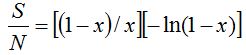 and are met (Fischer et al. 1943). According to this, values for S and N can be calculated from and are met (Fischer et al. 1943). According to this, values for S and N can be calculated from  and x amounts of ecological significance. Then, the values = 5000 and x = 0.995 were used (Magurran 2004) to obtain a community composed by 898341 individuals distributed among 26332 species. On the other hand, to work also on real data, the water sample of deep sea FS396.archaea was considered (Haegeman et al. 2013) (Huber et al. 2007), this sample is composed of 16316 sequences of 16S rRNA and its rarefaction curve reaches an asymptotic behavior at that size. The number of species present in this sample, which for this experience it was considered as a whole community, is 346. and x amounts of ecological significance. Then, the values = 5000 and x = 0.995 were used (Magurran 2004) to obtain a community composed by 898341 individuals distributed among 26332 species. On the other hand, to work also on real data, the water sample of deep sea FS396.archaea was considered (Haegeman et al. 2013) (Huber et al. 2007), this sample is composed of 16316 sequences of 16S rRNA and its rarefaction curve reaches an asymptotic behavior at that size. The number of species present in this sample, which for this experience it was considered as a whole community, is 346.
In both cases, the observed number of species was compared with the estimations obtained by the non-parametric statistics CHAO and ACE and these in turn with the estimations performed by AQS. For the sample obtained from the simulated population the development of the estimation was studied while the amount of simulated individuals increased and the Turing estimator value decreased. For the FS396.archaea sample five subsamples of six different sizes were taken and with each one of them 10 runs of the algorithm were performed in order to estimate the expected value which in turn estimates S. To the comparison of performance the evaluation of the extrapolation was added by means of (Chao et al. 2014).
Here,  is the richness of the sample of initial size n which is calculated from the same, is the richness of the sample of initial size n which is calculated from the same,  is the number of singletons in the sample of size n and is the number of singletons in the sample of size n and  is an estimation of the number of species not observed in the sample of size n. The ACE estimation was taken as value that actually is designed as an estimator of the total species in the community and not as an estimator of the missing species in the sample. Thus this last amount may even be overvalued. The m value is the number of individuals that are ideally added to extrapolate. In the case where m become very large is an estimation of the number of species not observed in the sample of size n. The ACE estimation was taken as value that actually is designed as an estimator of the total species in the community and not as an estimator of the missing species in the sample. Thus this last amount may even be overvalued. The m value is the number of individuals that are ideally added to extrapolate. In the case where m become very large 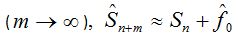 , will result, so such value could be taken as an upper bound of the extrapolation that, at first, it also will be considered in the analysis. Finally an evaluation of the respective coefficients of variation was performed. , will result, so such value could be taken as an upper bound of the extrapolation that, at first, it also will be considered in the analysis. Finally an evaluation of the respective coefficients of variation was performed.
III. RESULTS
For the simulated population built with the Fischer distribution of parameters =5000 and x=0.995, the experimental test consisted of applying the AQS on an initial sample of 1000 individuals performing different numbers of iterations. In each run the value that reached the probability of a new species was also obtained by cutting the simulation. Table 2 shows the results.
Based on the same sample of 1000 simulated individuals the performance of non-parametric estimators CHAO and ACE was compared with the AQS estimations obtained for increasing amounts of iterations. In turn, all of these results were compared with the actual number of species. Table 3 evidences the improvements that AQS produces in the estimation of richness regarding CHAO and ACE as the number of iterations increases. The series obtained searches an asymptotic value that not overtake S.
By using the set FS396.archaea to test the performance of AQS the estimation based on five samples of 160 individuals representing approximately 1% out of 16316 individuals within the community, is former studied. In each case, 10 runs of the algorithm were performed by comparing the AQS average estimations with the CHAO and ACE estimations, with the extrapolation and its bound, and the real value of the richness S=346. Figure 4 shows these results.
Then, five samples of each of the sizes 320, 640, 960, 1280 and 1600 were taken. On each sample 10 runs of the algorithm were performed establishing as estimation the average of the estimations for each run. The intention was to compare the estimations ACE and AQS with the actual known richness. Figure 5 shows the results obtained in each run for each sample and sample size.
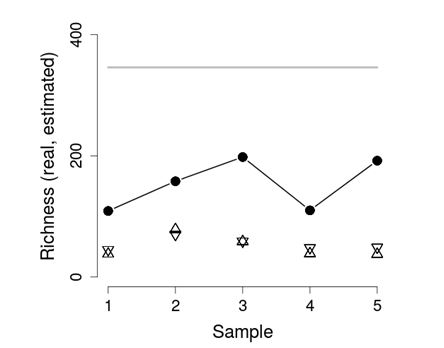 Fig. 4. Richness Estimation (sample size 160). The thick gray line is the real richness. The black circles are the AQS estimations, the triangles are the CHAO estimations and the invert triangles are the ACE estimations.
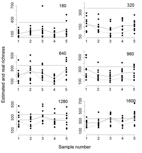 Fig. 5. Comparison between AQS and ACE estimations. The horizontal gray line is the real richness. The complete line is the AQS estimation and the dashed line is the ACE estimation. The number in the upper right corners is the sample size.
Although, in ecological practice, one community sample can be chosen for each sample size, each of the estimators was averaged in order to compare them in statistics terms. Thus, Figure 6 shows that the increase in sample size produces, as expected, a better average performance of all of them. Particularly, when the results are observed in percentage of richness obtained by AQS and ACE according to the percentage sample size with reference to the population, AQS shows one improvement in the estimation as shown in Table 4. Differences in percentage estimations in favor of AQS over 100% of the richness are, for the present case, those of Table 5. Even for very large percentage-wise sample sizes, it is noted that the AQS estimation produces an improvement over the non-parametric statistical ACE.
A study of the variability was additionally carried out by measuring the coefficient of variation to establish the stability of each one of the estimators obtained from the five samples of each sample size. As an AQS estimation the average obtained based on the 10 runs performed for each sample was taken. CHAO, ACE, Extrapolation and Bound Extrapolation values from each sample were considered and, as observed values, the amounts of species obtained in each one of the five samples for each size were taken. These latter values will show then the variability of the sample richness. Figure 7 shows these results. A detailed analysis of the results was performed in the following section.
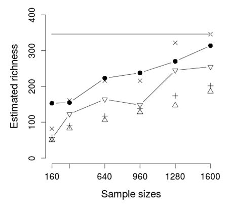 Fig. 6. Richness average estimation by size. The thick gray line is the real richness. The black circles are the AQS estimations, the triangles are the CHAO estimations and the invert triangles are the ACE estimations. The symbols x and + are the extrapolation ACE estimation and the bound extrapolation ACE estimation respectively.
IV. DISCUSSION
Using Fischer distribution to build a simulated population is based on the observation, particularly in certain marine biospheres, of statistically rare phylotypes that fit in this distribution (Galand et al. 2009). The simulation of the population based on such distribution requires to choose and x parameters that intervene in the calculation. The maximum number of individuals appearing in at least one cluster grows as the population size grows and potentially if an infinite population is assumed, it could be accepted that  . In this case the amount of species is . In this case the amount of species is 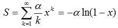 and the total number of individuals is . To deduce both formulas it has been taken into account that (Fischer et al. 1943). Furthermore, the amount is an intrinsic parameter of the richness of each population and can be used as an index of diversity (Magurran 2004). If values for the number of species S and n population size are established in advance, the value of x can be determined solving, by iterative methods, the equation and the total number of individuals is . To deduce both formulas it has been taken into account that (Fischer et al. 1943). Furthermore, the amount is an intrinsic parameter of the richness of each population and can be used as an index of diversity (Magurran 2004). If values for the number of species S and n population size are established in advance, the value of x can be determined solving, by iterative methods, the equation 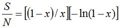 that expresses the ratio between the number of species and the population size. The parameter x then depends on this reason and in the practice is met without, of course, it can exceed the value 1 (Magurran 2004). that expresses the ratio between the number of species and the population size. The parameter x then depends on this reason and in the practice is met without, of course, it can exceed the value 1 (Magurran 2004).
Fig. 7. Comparison of coefficients of variation. The thick gray line is the real richness. The black circles are the AQS estimations, the triangles are the CHAO estimations and the invert triangles are the ACE estimations. The symbols x and + are the extrapolation ACE estimation and the bound extrapolation ACE estimation respectively.
Table 6 gives the values of the ratio calculated with different values of x assuming that the population size is 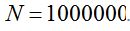 . Thence, is possible to obtain the number of species S and with it, the value of the parameter that can be calculated from N and x according to . Thence, is possible to obtain the number of species S and with it, the value of the parameter that can be calculated from N and x according to  . In all cases it is shown that . In all cases it is shown that  . As . As  is the first term of the log series, if x is close to 1, results approximately the expected number of species that appear once in the population, that is the minimum amount of species that can be considered rare. Also, when the ratio between the number of species and the population size decreases, as in some sense it expresses richness, also does it. In the practice the richness index can only be calculated from samples and in that case its value can be considered independent of the sample size when it has more than 1000 individuals. (Magurran 2004). is the first term of the log series, if x is close to 1, results approximately the expected number of species that appear once in the population, that is the minimum amount of species that can be considered rare. Also, when the ratio between the number of species and the population size decreases, as in some sense it expresses richness, also does it. In the practice the richness index can only be calculated from samples and in that case its value can be considered independent of the sample size when it has more than 1000 individuals. (Magurran 2004).
If an initial approximation of richness between 5000 and 30000 species is considered for a population of 1 million individuals, the corresponding values x and should range between and respectively. For the chosen parameters = 5000 and x = 0.995, the value  represents approximately the number of species of greatest rarity of the community. represents approximately the number of species of greatest rarity of the community.
These species represent 19% of the total. In turn, according to the simulated distribution, there would be 10% of species represented by two individuals, 6% with three individuals in the population and so on. In short; a significant proportion of rare species in the community is present.
When a sample of 1000 individuals out of a total community of 897,541 was selected, the results dumped in Table 2 allowed checking the growing effectiveness of the AQS estimation while the number of individuals added in a simulated way to the sample increased. Also here, the decrease to 0 of the Turing estimation of a new species could be seen. Table 3 shows the proportion of the real richness detected as the number of iterations increases. Upon reaching the 500000, the estimated percentage of the richness by AQS is 93%, which is a qualitatively different performance than the one provided by ACE (26%) and CHAO (25%) from the same sample.
To select the F396.archaea sample and use it as a test population its relatively large size was considered and the asymptotic form which, considered all individuals, presents its rarefaction curve (Haegeman et al. 2013). By selecting five samples out of 160 individuals the AQS estimation was higher than that obtained as a bound of extrapolation and almost double the estimates made by ACE, CHAO and its own extrapolation when a number of ideal individuals who tripled the sample size were added. is the maximum recommended value by adopting a statistical point of view to perform the extrapolation (Chao et al. 2014). However, the experience also allowed confirming that the best estimation provided by AQS barely reached half of the real richness. In this sense, each estimation was averaged considering the five samples to obtain a graph that illustrates the percentage of the estimated real richness per statistical. Table 7 shows marked differences between the average estimations and the actual value. The increase in sample size allowed reducing these differences. Figure 5 shows that for samples of 1600 individuals, about 10% of the population size, cases of very precise estimation and even overestimation occurred. In general terms, Figure 6 and table 4 confirm the improved performance of AQS compared to the non-parametric estimator ACE. An extrapolation behavior with similar to that of CHAO is also observed producing both underestimation of the richness.
The extrapolation bound is closer to the values obtained by AQS, especially when the sample size grows. However, for the smaller sample size AQS provides a better estimation. As expected, in addition, a more precise estimation occurs when the size of the original sample increases.
In spite of the analysis performed, the results always evidence the differences in the precision of the estimation obtained in the simulated case by the Fischer distribution and the real case analyzed, suggesting the study of other measures to account for the community diversity, especially in the case in which the analyses should be performed from a single sample.
Figure 7 analyzes the variability of different estimations. First, it should be pointed out the inherent variability of sampling. This can be appreciated by varying the amount of different species that appear in different samples. These are represented by a gray line and exhibit the lowest relative variation for all sample sizes. According to this, the increase of the relative variation for each type of estimation will be linked to the second source of variability that is the inherent to the method used to establish it. Non-parametric estimations reveal percentages of variation between 6% and 33% for CHAO and between 17% and 45% for ACE, with respective variation ranges of 27% and 28%. AQS reveals lower rates, between 8% and 25%, and in turn lower range of variation of the same, 17%. Thus the AQS estimation better appreciates the richness and with less variability.
V. CONCLUSIONS
• An alternative approach has been presented based on an experimental model that "fits" the enlargement process of the sample needed to better accurate the richness estimation. Such approach, related to the data mining, uses an initial subset to predict a parameter value of the community.
• The results have significantly improved the estimations of richness carried out based on models and assumptions of analytical and statistical type.
• Anyway, is once again clear the need to assess the biodiversity through various measures supplementing the knowledge of the community, while providing a more reliable assessment of their properties.
• Given the best, though still insufficient, performance achieved in the richness estimation according to the alternative approach proposed, its application to other measures that quantify the amount of information and the distribution of species in the community is suggested.
VI. REFERENCES
Armougom, F. and Raoult, D. 2009. Exploring Microbial Diversity Using 16S rRNA High-Throughput Methods. Journal of Computer Science & Systems Biology Volume 2(1): 074-092 (2009) – 074
Chao, A. 1984. Nonparametric estimation of the number of classes in a population.
Scand J Statist 11: 265-270.
Chao, A and Lee, S. 1992. Estimating the Number of Classes via Sample Coverage.
Journal of American Statistical Association. Volume 87. Issue 417.
Chao, A and Shen, T. 2003 Nonparametric estimation of Shannon’s index of diversity when there are unseen species in sample. Environmental and Ecological Statistics 10, 429-443.
Chao, A. Gotelli, N. J. Hsieh, T.C. Sander, E. L. Ma, K.H. Colwell, R. K. and Ellison A. M. 2014. Rarefaction and extrapolation with Hill numbers: a framework for sampling and estimation in species diversity studies. Ecological Monographs. 84 (1) 2014 pp.45-67.
Fischer, R. Corbett, S. and Williams, C. 1943. The Relation Between the Number of Species and the Number of Individuals in a Random Sample of an Animal Population. The Journal of Animal Ecology. British Ecological Society. Vol 12 N°1 (1943)
Galand, P. E. Casamayor, E. O. Kirchman, D. L. and Lovejoy, C. 2009. Ecology of the rare microbial biosphere of the Artic Ocean. PNAS. Vol. 106 no. 52 22427-22432.
Good, I. 1953. “The Population Frequencies of Species and Estimation of Population Parameters”. Biometrika. Vol 40 N° 3/4.
Gotelli, n and Colwell,R. 2001. Quantifying biodiversity: procedures and pitfalls in measurement and comparison of species richness. Ecology Letters. 4: 379-391
Haegeman, B. Hamelin, J. Motitarty, J. Neal, P. Dushoff, J. and Weitz, J. 2013 Robust estimation of microbial diversity in theory and in practice. ISME Journal 2013, 1-10
Hill, M. O. 1973. Diversity and Eveness: A Unifying Notation and Its Consequeces.
Ecology. Vol.54. No 2 pp 427-432.
Hill, T. Walsh, K. Harris, J. and Moffett, B. 2003. Using Ecological Diversity Measures with Bacterials Communities. FEMS.Microbiology Ecology 43 1-11
Hillis, D. M. Moritz, C. and Mable, B. K. 1996. Molecular Systematics. Second Edition, Sinauer Associates, Inc. Publishers. Sunderland, MA. USA.
Huber, J. A. Mark Welch, D. B. Morrison, H. G. Huse, S. M. Neal, P.R. Butterfield, D. and A. Sogin, M. L. 2007. Microbial Population Structures in the Deep Marine Biosphera. Science 318, 97(2007) DOI: 10.1126/science.1146689
Hughes, J. Hellmann, J. Ricketts, T. and Bohannan, B. 2001. Counting the uncountable: statistical approaches to estimating microbial diversity. Applied and Environmental Microbiology. 4399-4406.
Hughes,J and Hellman, J. 2005. The Application of Rarefaction Techniques to Molecular Inventories of Microbial Diversity. Methods in Enzymology. Vol 397.
Huse, S. M. Welch, D.M. Morrison, H.G. and Sogin, M.L. 2010. Ironing out the wrinkles in the rare biosphere through improved OTU clustering Environmental Microbiology (2010) 12(7), 1889–1898
Magurran, A. 2004. Measuring Biological Diversity. Blackwell Science Ltd.
Magurran, A and McGill, B.J. 2011. Biological Diversity. Oxford University Press.
Nádas, A. 1985. On Turing’s Formula for Word Probabilities. IEEE Transactions on Acoustics, Speech and Signal Processing. Vol ASSP-33 N° 6.
O’Hara, R. 2005. Species richness estimators: how many species can dance on de head of a pin. Journal of Animal Ecology. 74, 375.386
Roesch, L. Fulthorpe, R. Riva, A. Casella, G. Hadwin, A. Kent, A. Daroub, S. Camargo, F. Farmerie, W. and Triplett, E. 2007. Pyrosequencing enumerates and contrasts soil microbial diversity. The ISME Journal. 1, 283-290.
Schloss, P and Handelsman, J. 2005. Introducing DOTUR, a Computer Program for Defining Operational Taxonomic Units and Estimating Species Richness. Applies and Environmental Microbiology. pp 1501-1506
Schloss, P. and Handelsman,J. 2006. Toward a census of bacteria in soil. PLoS Computational Biology. Volume 2.
Schloss, P. 2010. The Effects of Alignment Quality, Distance Calculation Method, Sequence Filtering, and Region on the Analysis of 16S rRNA Gene-based Studies. PLoS Computational Biology 6(7): e1000844. doi:10.1371/Journal.pcbi.1000844.
Youssef, N. and Elshahed, M. 2008. Species richness in soil bacterial communities: A proposed approach to overcome sample size bias. Journal of Microbiological Methods. 75 86-91.
Recibido: 2017-06-28
Aprobado: 2017-07-10
Datos de edición: Vol.2 - Nro.1 - Art.1
Fecha de edición: 2017-08-15
URL: http://www.reddi.unlam.edu.ar
|
|